Why model?

class: center, middle, inverse, title-slide

# Why model?
## What If: Chapter 11
### Elena Dudukina
### 2021-04-15

---

# Welcome to Part II of Causal Inference Book
.pull-left[
![:scale 60%](Screenshot 2021-04-14 105528.jpg)
]
.pull-right[![:scale 70%](Screenshot 2021-04-14 105417.jpg)
]
---
# 11.1 Data cannot speak for themselves
- A: anti-retroviral therapy
- Y: CD4 cell count at the end of the study
- N: 16 individuals

- Estimator: `\(\hat{E}[Y|A=a]\)` (a function of the data) used to estimate the unknown populational parameter
- Consistent estimator: `\(\hat{E}[Y|A=a]\)` satisfies the criterion with the increased sample size the estimate is closer to the populational value `\(E[Y|A=a]\)`
- Possible estimators:
    - sample average of Y among those receiving `\(A=a\)` (a consistent estimator)
    - the Y value of the first observation in the dataset with `\(A=a\)` (not a consistent estimator)
---
# 11.1 Data cannot speak for themselves
.pull-left[
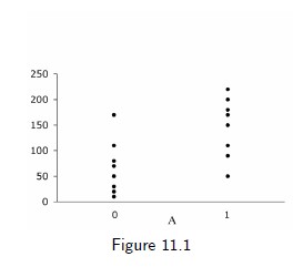
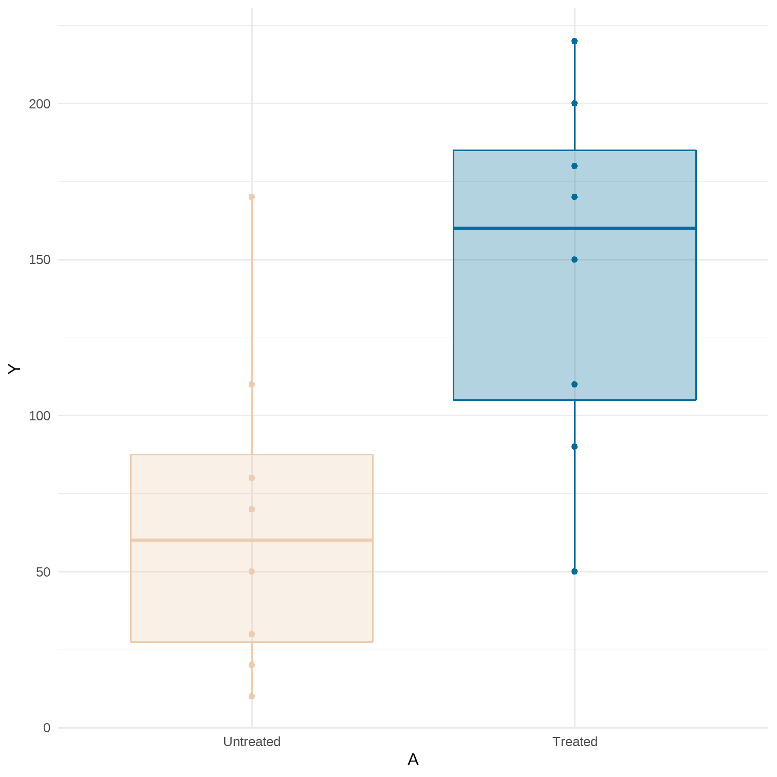
- Population mean in the treated is the sample average 146.25 for those with `\(A=1\)`

- Population mean in the untreated is the sample average 67.50 for those with `\(A=0\)`

- Under exchangeability between `\(A=1\)` and `\(A=0\)`, the average treatment effect (ATE) is `\(146.25 - 67.50 = 78.75\)`

]
.pull-right[
![:scale 70%](Screenshot 2021-04-14 122533.jpg)
]
---
# 11.1 Data cannot speak for themselves
.panelset[

.panel[.panel-name[Code]

```r
library(tidyverse)
library(magrittr)
# Sample averages by treatment level
# Data for Figure 11.1

A <- c(1, 1, 1, 1, 1, 1, 1, 1, 0, 0, 0, 0, 0, 0, 0, 0)
Y <- c(200, 150, 220, 110, 50, 180, 90, 170, 170, 30, 70, 110, 80, 50, 10, 20)

data <- tibble(A, Y) %>% 
  mutate(A = factor(A, levels = c("0", "1"), labels = c("Untreated", "Treated")))

p <- data %>% ggplot(aes(x = A, y = Y, color = A, fill = A)) +
  geom_point() +
  geom_boxplot(alpha = 0.3) +
  theme_minimal() +
  theme(legend.position = "none") +
  scale_color_manual(values = wesanderson::wes_palette(name = "Darjeeling2", n = 2)) +
  scale_fill_manual(values = wesanderson::wes_palette(name = "Darjeeling2", n = 2))
```
]

.panel[.panel-name[Output: means]

```r
data %>% group_by(A) %>% summarise(mean = mean(Y)) %>% kableExtra::kable()
```

<table>
 <thead>
  <tr>
   <th style="text-align:left;"> A </th>
   <th style="text-align:right;"> mean </th>
  </tr>
 </thead>
<tbody>
  <tr>
   <td style="text-align:left;"> Untreated </td>
   <td style="text-align:right;"> 67.50 </td>
  </tr>
  <tr>
   <td style="text-align:left;"> Treated </td>
   <td style="text-align:right;"> 146.25 </td>
  </tr>
</tbody>
</table>

]

.panel[.panel-name[Output: box plot]
<img src="index_files/figure-html/unnamed-chunk-4-1.png" width="504" />

]

]
---
# 11.1 Data cannot speak for themselves
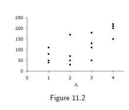
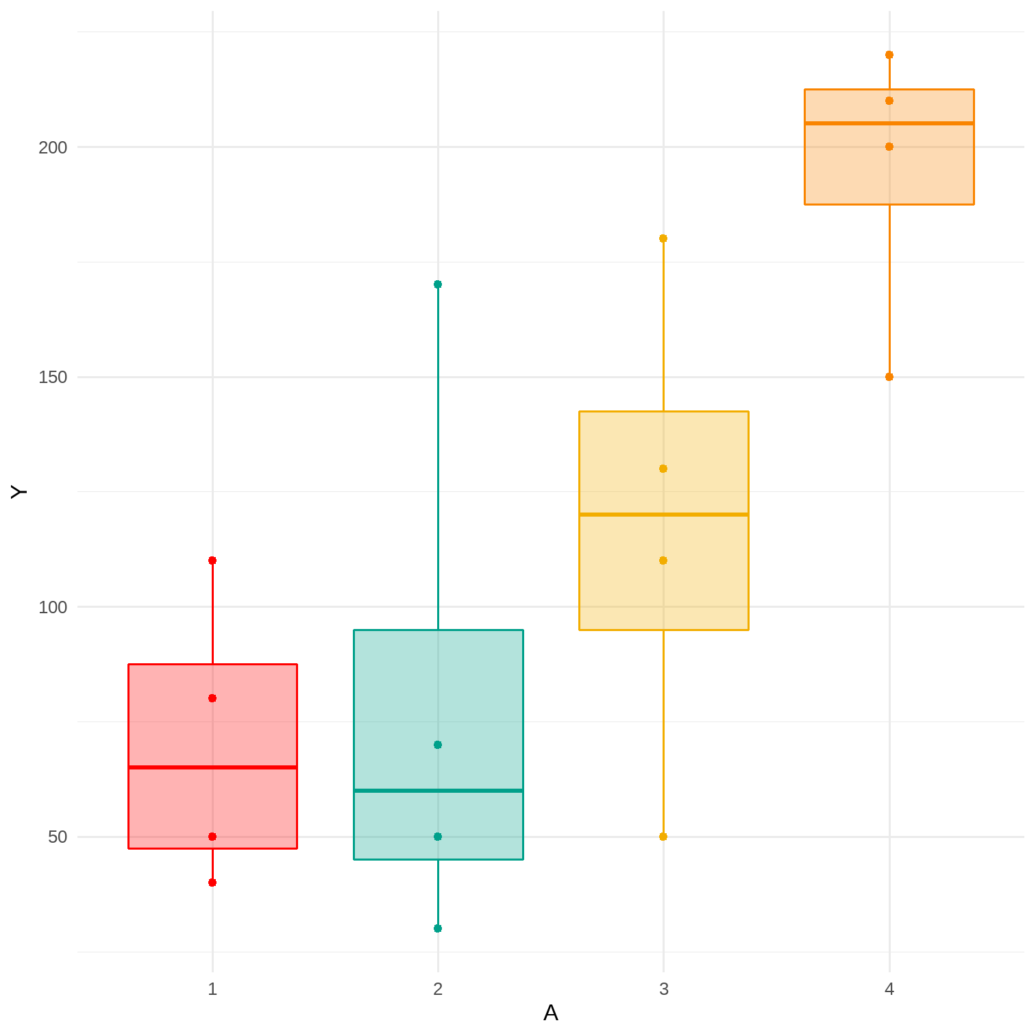
.pull-left[- A is polytomous variable
    - no treatment (A = 1)
    - low-dose treatment (A = 2)
    - medium-dose treatment (A = 3)
    - high-dose treatment (A = 4)
    
- Probability of getting any treatment level is 0.25

]

.pull-right[
![](Screenshot 2021-04-14 133622.jpg)
]

---
# 11.1 Data cannot speak for themselves

.panelset[

.panel[.panel-name[Code]

```r
# Sample averages by treatment level
# Data for Figure 11.2
A <- c(1, 1, 1, 1, 2, 2, 2, 2, 3, 3, 3, 3, 4, 4, 4, 4)
Y <- c(110, 80, 50, 40, 170, 30, 70, 50, 110, 50, 180, 130, 200, 150, 220, 210)

data <- tibble(A, Y) %>% 
  mutate(A = factor(A))

p <- data %>% ggplot(aes(x = A, y = Y, color = A, fill = A)) +
  geom_point() +
  geom_boxplot(alpha = 0.3) +
  theme_minimal() +
  theme(legend.position = "none") +
  scale_color_manual(values = wesanderson::wes_palette(name = "Darjeeling1", n = 4)) +
  scale_fill_manual(values = wesanderson::wes_palette(name = "Darjeeling1", n = 4))
```
]

.panel[.panel-name[Output: means]

```r
data %>% group_by(A) %>% summarise(mean = mean(Y)) %>% kableExtra::kable()
```

]

.panel[.panel-name[Output: box plot]
<img src="index_files/figure-html/unnamed-chunk-7-1.png" width="504" />

]

]
---
# 11.1 Data cannot speak for themselves
.pull-left[
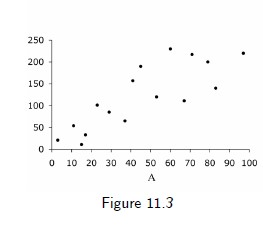
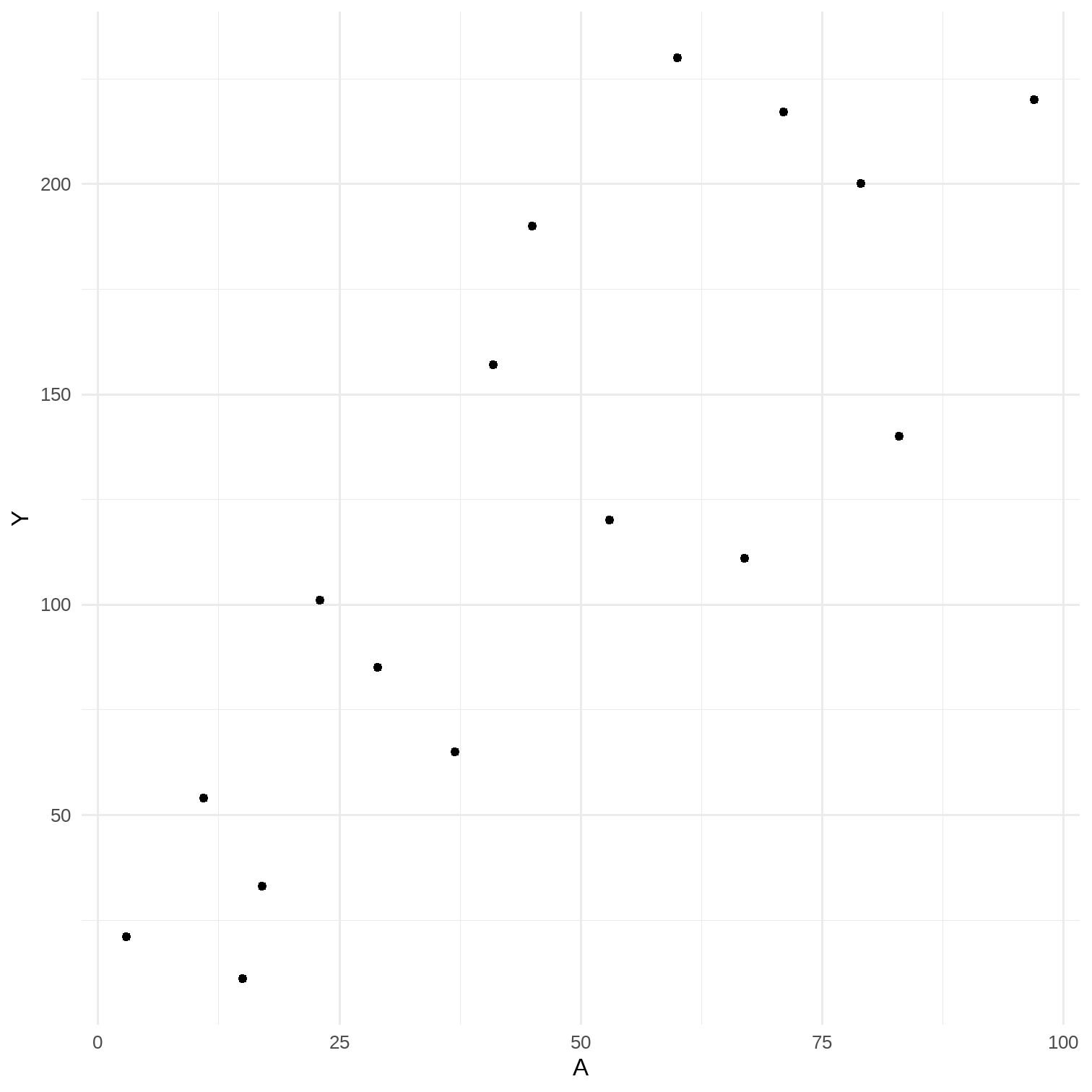
- A is a dose treatment in in mg/day
- Values [0;100]
- A continuous variable is a categorical variable with infinite number of categories
- estimate, in the target population, the mean of the outcome Y among individuals with treatment level A = 90
]

.pull-right[
![](Screenshot 2021-04-14 134948.jpg)
]
---
# 11.1 Data cannot speak for themselves
.panelset[

.panel[.panel-name[Code]

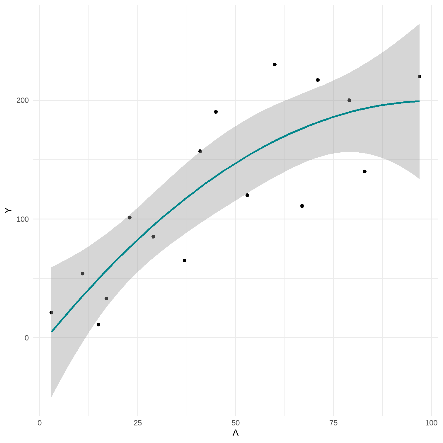
```r
# 2-parameter linear model
# Data for Figures 11.3

A <- c(3, 11, 17, 23, 29, 37, 41, 53, 67, 79, 83, 97, 60, 71, 15, 45)
Y <- c(21, 54, 33, 101, 85, 65, 157, 120, 111, 200, 140, 220, 230, 217, 11, 190)

data <- tibble(A, Y)

rm(A, Y)

res_lm <- lm(Y ~ A, data = data) %>% 
  broom::tidy(., conf.int = T) %>% 
  select(1, 2, 6, 7)

p <- data %>% 
  ggplot(aes(x = A, y = Y)) +
  geom_point() +
  theme_minimal()
```
]

.panel[.panel-name[Output: models]

```
## # A tibble: 2 x 4
##   term        estimate conf.low conf.high
##   <chr>          <dbl>    <dbl>     <dbl>
## 1 (Intercept)    24.5    -21.2      70.3 
## 2 A               2.14     1.28      2.99
```

]

.panel[.panel-name[Output: plot]
<img src="index_files/figure-html/unnamed-chunk-10-1.png" width="504" />
]
]
---
# 11.2 Parametric estimators of the conditional mean
- Aim: to estimate mean of Y among individuals with treatment level A = 90, or `\(E[Y|A=90]\)`
- Y ~ Normal(A, `\(\epsilon\)`) (Y is a function of A with some error term)
- The mean of Y changes from some value `\(\theta_0\)` by `\(\theta_1\)` units per unit of treatment A: `\(E[Y|A]=\theta_0 + \theta_1A\)`
- The shape of conditional mean `\(E[Y|A]\)` is determined by this equation - linear mean model
- `\(\theta_0\)` and `\(\theta_1\)` are parameters of the model
- If model describes the expectation with a finite number of parameters, the model is parametric
---
.panelset[

.panel[.panel-name[lm figure code]

```r
# Figure 11.4
p <- data %>% 
  ggplot(aes(x = A, y = Y)) +
  geom_point() +
  geom_smooth(method = lm, color = "#00868B") +
  theme_minimal()
```
]
.p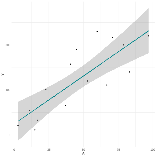anel[.panel-name[lm figure]

```r
p
```

![](index_files/figure-html/unnamed-chunk-12-1.png)
]
.panel[.panel-name[lm parameters]

```r
lm(Y ~ A, data = data) %>% 
  broom::tidy(., conf.int = T) %>% 
  select(1, 2, 6, 7)
```

]

.panel[.panel-name[predicted value at A=90]

```r
24.546369 + 2.137152*90
```

```
## [1] 216.89
```
]
]
---
# 11.2 Parametric estimators of the conditional mean
- A model restricts the joint distribution of the data
- Parametric models come with the assumptions
- The inferences are valid only when the model is correctly specified
- Assumption of no model misspecification for the model-based causal inference
---
# 11.3 Nonparametric estimators of the conditional mean
For dichotomous treatment A:
- `\(E[Y|A]=\theta_0 + \theta_1A\)`
- `\(E[Y|A=1] = E[Y|A=0] + \theta_1\)`
- Saturated model
- "Model is saturated whenever the number of parameters in a conditional mean model is equal to the number of unknown conditional means in the population"
- "When a model has only a few parameters but it is used to estimate many population quantities, it is parsimonious"
---
# 11.4 Smoothing
- Linear model with quadratic term `\(A^2\)` (or other polynomials: `\(...\)`, `\(A^{15}\)`)
- `\(E[Y|A]=\theta_0 + \theta_1A + \theta_2A^2\)`
- The more parameters the model has, the less smooth the curve is
---
# 11.4 Smoothing
.panelset[

.panel[.panel-name[lm with quadratic term]

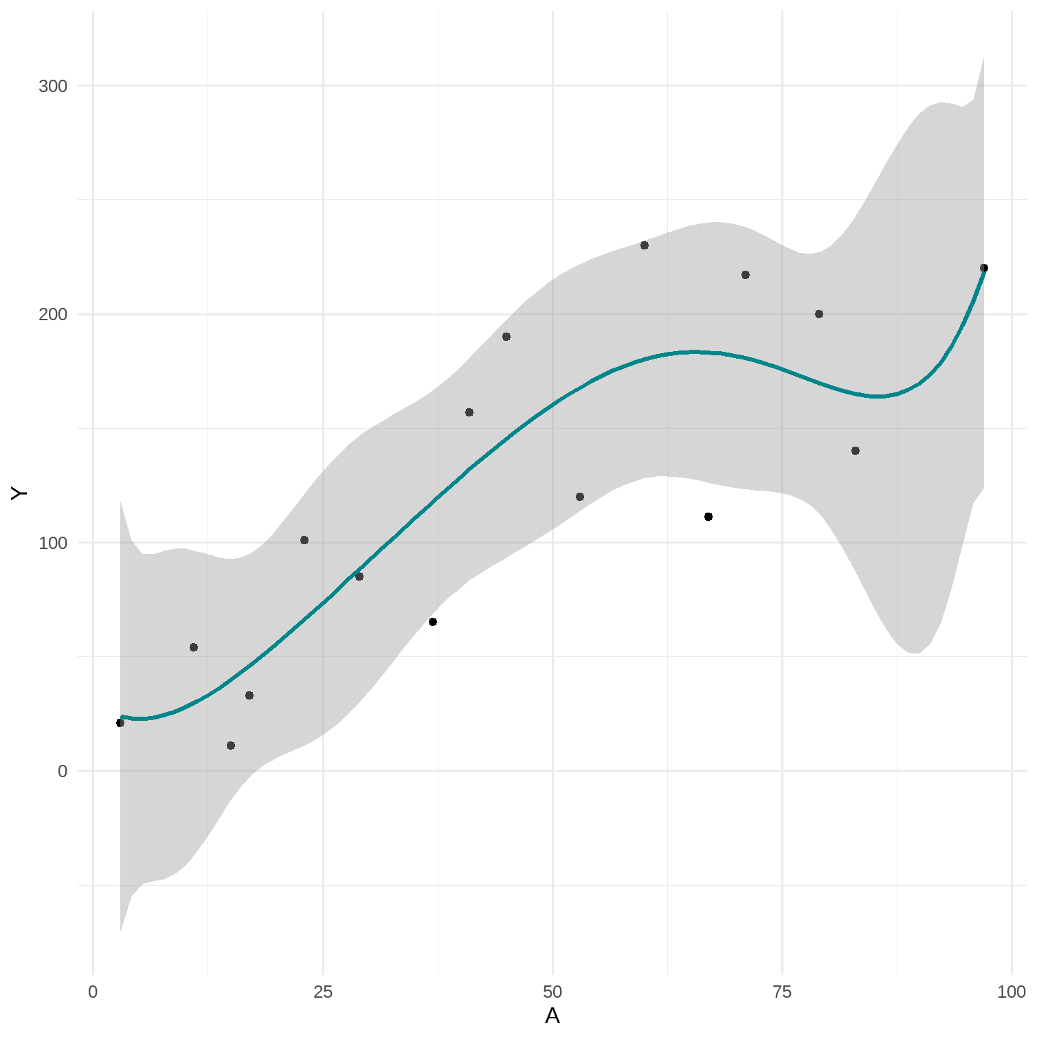
```r
data %<>% mutate(A_sq = A*A)

lm(Y ~ A + A_sq, data = data) %>% 
  broom::tidy(., conf.int = T) %>% 
  select(1, 2, 6, 7)
```

```
## # A tibble: 3 x 4
##   term        estimate conf.low conf.high
##   <chr>          <dbl>    <dbl>     <dbl>
## 1 (Intercept)  -7.41   -76.0      61.2   
## 2 A             4.11     0.800     7.41  
## 3 A_sq         -0.0204  -0.0535    0.0127
```

```r
# predict by hand
-7.40687745 + 4.10722663*90 -0.02038477*90^2
```

```
## [1] 197.1269
```
]

.panel[.panel-name[Code]

```r
# 3 parameters
p <- data %>% 
  ggplot(aes(x = A, y = Y)) +
  geom_point() +
  theme_minimal() + 
  stat_smooth(method = "glm", formula = y ~ poly(x, 2), color = "#00868B")
# 7 parameters
p2 <- data %>% 
  ggplot(aes(x = A, y = Y)) +
  geom_point() +
  theme_minimal() + 
  stat_smooth(method = "glm", formula = y ~ poly(x, 6), color = "#00868B")
```
]
.panel[.panel-name[figure: quadratic term]
<img src="index_files/figure-html/unnamed-chunk-17-1.png" width="504" />
]

.panel[.panel-name[figure: polynomial of degree six]
<img src="index_files/figure-html/unnamed-chunk-18-1.png" width="504" />
]
]
---
# 11.5 The bias-variance trade-off
- Under 2-parameter model the prediction for CD4 cell count given A=90 was 216.9 and under 3-parameter model it was 197.1
- 3-parameter model is correctly specified under both straight line and curvelinear scenarios
- More parameters, less restrictions model implies
- Less smooth models provide less biased, but more imprecise result (estimate with a larger variance)

---
# References
Hernán MA, Robins JM (2020). Causal Inference: What If. Boca Raton: Chapman & Hall/CRC (v. 31mar21)